Voice Spectrograph and Speaker Identification

Introduction

The human voice transmits information beyond the words that are spoken. Within the acoustical framework is physiological and behavioural information that is sufficiently distinctive to suggest that voices can be used to identify people as fingerprints can (Gregory, 1986). The premise is that voice spectrograph, which transforms the sound energy of speech into a visual pattern called a spectrogram, and the whole discipline of speaker identification (SID), which employs acoustic and statistical modelling to identify a speaker, are complementary. The development of voice spectrograph from the Bell Telephone Laboratories research in the 1940s brought it into the courtroom in the mid-1960s and was a subject of decades of legal debate over its scientific validity (Gregory, 1986).  In parallel to these legal developments, engineering research has shifted from a manual approach of comparing spectrograms to statistical pattern recognition and, more recently, a deep learning approach of speaker modelling (Tirumala & Shahamiri, 2016). 

Fundamentals of Voice and Speech

Physiological traits (the size and shape of the vocal cavities and articulators-throat, nose, mouth, tongue and jaw) as well as behavioural, or learned, speech patterns are correlated with the speaker’s identity (Furui, 1994; Gregory,1986). Voice identification theory is based on two assumptions; 1) that the anatomical differences between speakers result in measurable differences between their voices when they say the same sound (interspeaker variation) and that 2) these voices of the same person will have some temporal variation due to colds, fatigue, stress, or aging, but the pattern remains more or less stable (intraspeaker variability) (Gregory, 1986). Valid identification of the spectra is possible only when interspeaker variability is always greater than intraspeaker variability. Energy in speech has been said to occur on two planes; one that the speaker can intentionally modify and one that is largely unwitting and cannot be disguised. This theoretical basis is intuitively satisfying, but some argue that uniqueness of the human voice has never been established via controlled empirical research (Gregory, 1986).

Voice Spectrograph: Principle and working.

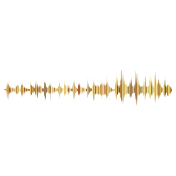
A spectrograph is a method of mapping the acoustic signal into a three-dimensional picture: X axis – time, Y axis – frequency and the darkness of the shading describes the intensity of the signal. High-amplitudee frequency bands, called formants, are seen as dark bands, in which the spacing and pattern of these bands change depending on the sound made. The traditional forensic exam involves selecting equivalent words or phrases from a known and an unknown recording, creating a spectrogram of each word or phrase, comparing the similarity of the spectrograms on the following parameters: the mean frequency of the formants, their width, the spacing between the vertical striations, the slope of the diphthong transitions, and the overall rate of speech, and making a final aural (listening) comparison. Usually, 10-20 points of concordance are required, and there is no standard number of points that is agreed. The technique compares the message; the phonetic content of an utterance can be very similar between different speakers saying the exact same word; therefore, visual pattern matching alone is very prone to misinterpretation (Gregory, 1986). This weakness has led to a change in forensic practice today to use likelihood-ratio-based, statistically calibrated methods, rather than just visual comparison (Phonexia, n.d.).

Speaker Identification Techniques

Automatic speaker recognition (ASR) systems formalize the identification problem as a two-part pattern-recognition problem: the enrolment (training) stage, where characteristic features are extracted from the voice of the speaker to construct a reference model; and the matching stage, where a test utterance is matched to stored models to make an identification or verification decision (Tirumala & Shahamiri, 2016). In this broad class of methods, many feature extraction, modelling and classification methods have been developed, ranging from manual spectrogram reading to fully automatic deep neural architectures.

• Text-dependent vs text-independent techniques.

SID can be broadly divided into two categories, text-dependent recognition and text-independent recognition. Text-dependent systems are systems in which the speaker says a specific or predetermined key word/sentence, which is the same at enrollment and during testing. The time axis of the training and test utterances can be aligned phoneme-by-phoneme, resulting in comparatively high accuracy and simple architectures, but this is not robust to playback attacks unless the system randomly chooses a new sentence for each session (“text-prompted” approach). For text-independent systems, no actual text is set; the speaker can say whatever he wants,s and the system is required to identify the speaker, regardless of content. More flexible, and not so easily mimicked by a fixed phrase; it also loses the ability to model speech at the word or sentence level, and has to be based on the long-term statistical characteristics of the voice (Furui, 1994).

•  Feature Extraction Techniques 

The effectiveness of any SID system relies crucially on the features extracted from the raw acoustic signal: these features need to have discriminative information sufficient to distinguish speakers, yet not so much that it gives away irrelevant variations like background noise (Tirumal & Shahamiri, 2016).

1. LPC-derived cepstral coefficients: The spectral envelope of speech was represented by the first-order speech model, linear predictive coding (LPC) cepstral coefficients, and the second-order LPC regression coefficients (delta- and delta-delta-cepstral coefficients) for spectral dynamics between speech frames, in early automatic systems (Furui, 1994).
2. Mel-Frequency Cepstral Coefficients (MFCCs). In both SR and SID, the most popular feature. They are obtained by applying a Fourier transform to short frames of the signal and mapping the spectrum onto the mel scale, which models the human auditory function of frequency perception, and explicitly models the design of the filter-bank used to calculate MFCCs (Tirumal & Shahamiri, 2016).
3. Formant- and spectrogram-based features: In the classic (not automatic) spectrographic analysis, the examiner compares the formant frequencies, the formant widths, the distance between striations, the diphthong slope and the speed of speech directly from the visual spectrogram, while also comparing the sounds aurally (Gregory, 1986). This approach is more subjective and examiner-dependent than the statistical feature extraction approach.
4. Instead of working directly with the high-dimensional set of features in individual frames, i-vector techniques employ front-end factor analysis to reduce the dimensionality of the “supervector” (typically over 1000 dimensions) into a low-dimensional vector (typically 400–600 dimensions) that represents speaker-specific characteristics; this reduction allows for more efficient and robust subsequent modelling.

•  Template-Matching Methods

The earliest SID systems were based on the Dynamic Time Warping (DTW) approach, which is a kind of spectral template-matching (STM) technique using short-term feature vectors as the stored reference template. These systems dynamically align the time axis of a test utterance to a stored reference template, a nonlinear alignment technique, to compensate for the natural variation in speaking rate. Distance between aligned sequences is summed and compared to a threshold for making a verification decision. DTW-based systems are easy to compute, but are only able to deal with the variations of vocabulary and are less suitable for long-term voice variations as compared to statistical approaches, which are limited to applications that rely on a fixed vocabulary and are not text-dependent (Furui, 1994).

•  Statistical pattern recognition methods 

1. Vector Quantisation (VQ): VQ-based methods are used to compress training feature vectors of a speaker into a small “codebook” of representative feature vectors without having to store and compare all of the speaker’s training vectors directly. An unknown utterance is vector-quantised by all reference speaker codebooks, and the accumulated quantisation error is used for the identification decision. Separate codebooks are usually constructed for voiced and unvoiced speech segments, taking advantage of both the spectral and pitch information (Furui, 1994).
2. Gaussian Mixture Models (GMMs): GMMs are based on the assumption that a speaker feature vector distribution can be modelled as a weighted sum of multivariate Gaussian densities, and are useful in cases of text-independent recognition where no prior knowledge of what is being spoken is available (Gregory, 1986; Shahamiri, 2016). GMMs can be considered as an extension of VQ where the assignment of the hard clusters is replaced by a soft cluster assignment.

• Spatial-Temporal Structure of Speech:  

The spatio-temporal structure of speech is modelled by Hidden Markov Models (HMMs), which are well suited to model spatio-temporal changes in the spectral characteristics. It is well known that HMM-based techniques such as ergodic HMMs that include transitions between all HMM states for modelling broad phonetic categories have better recognition accuracy than DTW-based techniques and are routinely used as the basis for the likelihood scoring that is used with text-dependent recognition (Furui, 1994).  Text-dependent recognition is generally performed by HMMs, which are trained to use prior information about the spoken text to create likelihood functions, while text-independently, based on i-vectors, GMMs adapted from a Universal Background Model (UBM) are more frequently used (Tirumal & Shahamiri, 2016).

Normalize scores and distances.

Raw similarity/distance scores have not been used directly in most instances because the signal characteristics differ significantly between recording sessions, depending on a number of factors such as channel conditions, microphone type, and the speaker’s own intersession variability. Instead, likelihood-ratio normalization compares the probability of the observed features for the claimed speaker to that of a “cohort” of representative impostor speakers, and a posteriori-probability normalization compares against the probability of the features for all the reference speakers, including the claimed speaker (Furui, 1994).

Both methods have been demonstrated to significantly enhance speaker separability and decrease the requirement for speaker- or text-dependent thresholds.

Approaches related to neural networks and deep learning.

Most recent generation of SID techniques uses deep neural architectures for feature extraction, classification or both at once:

1. DNN as feature extractor: A deep neural network is trained at the acoustic-frame level, and the activation values of the last hidden layer (not a SoftMax output) are added across the frames to obtain a concise representation of the speaker: the d-vector is similar to an i-vector but is learned directly from supervised training.
2. DNN as classifier: Conventional features, e.g., MFCCs arranged as stacked frames with temporal context around them, are input to an utterance-level DNN which outputs a probability distribution over speaker identities for each frame, which is averaged, or passed on to a second DNN, to get an utterance-level decision.
3. Deep Belief Networks (DBNs): DBNs are a stack of multiple layers of Restricted Boltzmann Machines trained unsupervised or semi-supervised; in particular, when labelled data is limited, or the system is required to make generalizations on previously unseen (“open-set”) speakers, as in Universal DBN (UDBN) architectures that operate directly on i-vectors.
4. Stacked Bottleneck Features (SBN): These architectures feed MFCC features into a “Bottleneck Neural Network” that has a deliberately small hidden layer, and then extract the bottleneck activations as powerful input features for a second cascaded network, which outperform single-stage bottleneck approaches.
5. Convolutional and hybrid architectures: Convolution and sub-sampling operations are applied in CNNs to identify features in a hierarchical fashion automatically, while phonetically aware DNNs have been used to replace the GMM-based posterior models in the construction of i-vectors, and are shown to produce better results than GMM-based models.

In all the benchmarks, the DNN-based architectures have performed better than the traditional GMM/MFCC pipeline, especially in the presence of noise or when the test utterances are short. This is because the DNN can be trained layer-wise, where each layer learns increasingly abstract, speaker-discriminative representations (Tirumal & Shahamiri, 2016).

Forensic Investigations: Applications.

Voice spectrograph has been employed in the identification and in corroboration of identity in cases of criminal prosecution, and in a rare number of instances in the exculpation of the defendant. The early rulings were varied, with most federal courts accepting spectrographic evidence as relevant and reliable and many state courts rejecting it in light of the general-acceptance standard of Frye. Outside the courtroom, spectrographic and voiceprint science has been used as a helpful investigative tool in probable cause investigations and in probation revocation hearings, even when there were disputes regarding trial admissibility (Gregory, 1986). 

Historically, the U.S. Department of Justice has commented that the majority of courts faced with the question determined that voiceprint evidence was admissible. Since then, however, the field has progressed significantly, and agencies have shifted away from the traditional visual spectrographic method of evidentiary analysis to statistically based automatic forensic voice comparison techniques that yield likelihood ratio conclusions instead of a match/not match classification (Phonexia, n.d.; UC Irvine, n.d.).

More recent Daubert decisions, like United States v. Angleton (2003), have held that the testimony of a spectrographist is not admissible without the provision of any eempirically basederror rate (UC Irvine, n.d.).

References:

1. UC Irvine. (n.d.). Morrison & Thompson: Assessing the admissibility of a new generation of forensic voice comparison testimony [PDF]. eScholarship. Retrieved July 30, 2026, from https://escholarship.org/content/qt5239p0tz/qt5239p0tz.pdf
2. U.S. Department of Justice. (n.d.). Justice Manual §258: Admissibility of spectrograms (voice prints). Retrieved July 30, 2026, from https://www.justice.gov/archives/jm/criminal-resource-manual-258-admissibility-spectrograms-voice-prints
3. Sharon E. Gregory, Voice Spectrography Evidence: Approaches to Admissibility, 20 U. Rich. L. Rev. 357 (1986). Available at: http://scholarship.richmond.edu/lawreview/vol20/iss2/6
4. Furui, S. (1996). An overview of speaker recognition technology. Automatic Speech and Speaker Recognition: Advanced Topics, 31-56.
5. Tirumala, S. S., & Shahamiri, S. R. (2016, November). A review on deep learning approaches in speaker identification. In Proceedings of the 8th International Conference on Signal Processing Systems (pp. 142-147).